 trevor simonton
how does the huffman tree work in word2vec?
There are two major approaches to training the word2vec model. One is the so called “hierarchical softmax” and the other is a process called “Noise Contrastive Estimation”. For the “hierarchical softmax” method, a Huffman binary tree is used [1,2].
Before reading about word2vec, I was familiar with Huffman coding as a means of lossless data compression, but I was confused about how exactly the tree is constructed, and then how it is used in word2vec’s “hierarchical softmax” method.
I wrote this post to explain what I found.
part 1: tree construction
word2vec’s CreateBinaryTree()
The magic is in the source code:
void CreateBinaryTree() {
  long long a, b, i, min1i, min2i, pos1, pos2, point[MAX_CODE_LENGTH];
  char code[MAX_CODE_LENGTH];
  long long *count = (long long *)calloc(vocab_size * 2 + 1, sizeof(long long));
  long long *binary = (long long *)calloc(vocab_size * 2 + 1, sizeof(long long));
  long long *parent_node = (long long *)calloc(vocab_size * 2 + 1, sizeof(long long));
  for (a = 0; a < vocab_size; a++) count[a] = vocab[a].cn;
  for (a = vocab_size; a < vocab_size * 2; a++) count[a] = 1e15;
  pos1 = vocab_size - 1;
  pos2 = vocab_size;
  // Following algorithm constructs the Huffman tree by adding one node at a time
  for (a = 0; a < vocab_size - 1; a++) {
    // First, find two smallest nodes 'min1, min2'
    if (pos1 >= 0) {
      if (count[pos1] < count[pos2]) {
        min1i = pos1;
        pos1--;
      } else {
        min1i = pos2;
        pos2++;
      }
    } else {
      min1i = pos2;
      pos2++;
    }
    if (pos1 >= 0) {
      if (count[pos1] < count[pos2]) {
        min2i = pos1;
        pos1--;
      } else {
        min2i = pos2;
        pos2++;
      }
    } else {
      min2i = pos2;
      pos2++;
    }
    count[vocab_size + a] = count[min1i] + count[min2i];
    parent_node[min1i] = vocab_size + a;
    parent_node[min2i] = vocab_size + a;
    binary[min2i] = 1;
  }
  // Now assign binary code to each vocabulary word
  for (a = 0; a < vocab_size; a++) {
    b = a;
    i = 0;
    while (1) {
      code[i] = binary[b];
      point[i] = b;
      i++;
      b = parent_node[b];
      if (b == vocab_size * 2 - 2) break;
    }
    vocab[a].codelen = i;
    vocab[a].point[0] = vocab_size - 2;
    for (b = 0; b < i; b++) {
      vocab[a].code[i - b - 1] = code[b];
      vocab[a].point[i - b] = point[b] - vocab_size;
    }
  }
  free(count);
  free(binary);
  free(parent_node);
}
Easy, right? Well… for me, getting my head around this code involved stepping through it, line by line, while drawing a picture of memory.
As I started to draw my picture of a miniature example, I realized I could alter the code to output some animation callbacks. This is what I did to generate the animation that I’ll use later in this post.
background info
(globals, initializations, definitions)
Note that this code depends on a few global variables that are used in word2vec. Namely, vocab and vocab_size.
These are defined elsewhere in the file:
vocab = (struct vocab_word *)calloc(vocab_max_size, sizeof(struct vocab_word));So vocab is just a dynamic array of vocab_word structs:
struct vocab_word {
  long long cn;
  int *point;
  char *word, *code, codelen;
};
vocab_size grows as the vocabulary is read from an input file.
setting up an example
the input vocabulary file
For the rest of the example, I’ll use this input file:
how much wood would a wood chuck chuck if a wood chuck could chuck wood
program used to view tree results
In order to view the result of the CreateBinaryTree() function, I created a small C program that uses some of word2vec’s functions. The gist of this program is as follows:
void printVocab() {
  int i,a;
  for (i = 0; i < vocab_size; ++i) {
    for (a = 0; a < vocab[i].codelen; ++a) {
      vocab[i].code[a] = vocab[i].code[a] == 1 ? '1' : '0';
    }
    printf("%s: \n\tcount: %d\n\tpoint: arr\n\tcode: %s\n\tcodelen: %d\n",
        vocab[i].word, vocab[i].cn, vocab[i].code, vocab[i].codelen);
  }
}

int main() {
  strcpy(train_file, "words.txt");

  vocab = (struct vocab_word *)calloc(vocab_max_size, sizeof(struct vocab_word));
  vocab_hash = (int *)calloc(vocab_hash_size, sizeof(int));
  LearnVocabFromTrainFile();
  CreateBinaryTree();
  printVocab();
}
In main() I’m just initializing my vocabulary as it is initialized in word2vec’s original C implementation.
I then call on the LearnVocabFromTrainFile() which is also in the original C implementation to populate my array of vocab_word structs.
I then call CreateBinaryTree(), which is the function at the top of this post, and is also in the original C implementation.
My printVocab() function then simply prints the vocab array out to stdout.
running the example
program output
When using the wood chuck words above (saved to “words.txt”), we get this:
Learn vocab from train file...
Vocab size: 9
Words in train file: 16
</s>:
	count: 1
	point: arr
	code: 10
	codelen: 2
wood:
	count: 4
	point: arr
	code: 01
	codelen: 2
chuck:
	count: 4
	point: arr
	code: 00
	codelen: 2
a:
	count: 2
	point: arr
	code: 1111
	codelen: 4
how:
	count: 1
	point: arr
	code: 1100
	codelen: 4
much:
	count: 1
	point: arr
	code: 11101
	codelen: 5
would:
	count: 1
	point: arr
	code: 11100
	codelen: 5
if:
	count: 1
	point: arr
	code: 11011
	codelen: 5
could:
	count: 1
	point: arr
	code: 11010
	codelen: 5
The count properties are set by LearnVocabFromTrainFile(), and the point, code and codelen properties are set during CreateBinaryTree().
what just happened?
The LearnVocabFromTrainFile() builds a hash table of word structs. Using this hash table, the function counts repeat occurrences of unique words.
The “learn” function also builds vocab, which gives each unique word in the vocabulary an index in an array.
In this example, after the “learn” function runs, the vocab array looks like this:
0: </s>
1: wood
2: chuck
3: a
4: how
5: much
6: would
7: if
8: could
Note that this array is sorted, with the most frequently occurring items appearing at the start of the array. (This is handled by SortVocab() which is called by LearnVocabFromTrainFile() after all of the words are hashed and counted.)
Also note that </s>, or the “end of sentence token” is given a special place at the front of this array, regardless of its count.
After the vocabulary is ingested from the input file, CreateBinaryTree() is called, and we build our Huffman tree.
back to CreateBinaryTree()
The first giant chunk of this function is just setting aside some space in memory:
  long long a, b, i, min1i, min2i, pos1, pos2, point[MAX_CODE_LENGTH];
  char code[MAX_CODE_LENGTH];
  long long *count = (long long *)calloc(vocab_size * 2 + 1, sizeof(long long));
  long long *binary = (long long *)calloc(vocab_size * 2 + 1, sizeof(long long));
  long long *parent_node = (long long *)calloc(vocab_size * 2 + 1, sizeof(long long));
All of these are local variables that will be used to build an array called parent_node. This array will describe the parent-child relationship of each node in our binary tree.
This tree includes nodes that are not leaves. That is why we have vocab_size * 2 + 1 entries in our arrays. Non-leaf nodes are not part of the vocabulary. The leaf nodes of our tree are complete words that are found in the vocabulary. The most common words have the shortest paths from root to leaf.
Notice these initializers:
  for (a = 0; a < vocab_size; a++) count[a] = vocab[a].cn;
  for (a = vocab_size; a < vocab_size * 2; a++) count[a] = 1e15;
The count of each word in vocab is passed to the count array, and then we initialize up to vocab_size * 2 slots in this array to a maximum value. These extra slots are the parent, non-leaf nodes in our Huffman tree.
The core of the tree construction algorithm is this part of the function:
  pos1 = vocab_size - 1;
  pos2 = vocab_size;
  // Following algorithm constructs the Huffman tree by adding one node at a time
  for (a = 0; a < vocab_size - 1; a++) {
    // First, find two smallest nodes 'min1, min2'
    if (pos1 >= 0) {
      if (count[pos1] < count[pos2]) {
        min1i = pos1;
        pos1--;
      } else {
        min1i = pos2;
        pos2++;
      }
    } else {
      min1i = pos2;
      pos2++;
    }
    if (pos1 >= 0) {
      if (count[pos1] < count[pos2]) {
        min2i = pos1;
        pos1--;
      } else {
        min2i = pos2;
        pos2++;
      }
    } else {
      min2i = pos2;
      pos2++;
    }
    count[vocab_size + a] = count[min1i] + count[min2i];
    parent_node[min1i] = vocab_size + a;
    parent_node[min2i] = vocab_size + a;
    binary[min2i] = 1;
  }
Step through the below animation for a walkthrough of how this works in our “wood chuck” example. Each white column in this table represents one of our 8 words. (Check the index to word map above).
The “grayer” columns (indices 9 to 18) are used for non-leaf nodes in the tree.
You can either click “play” and watch the magic happen, or you can click “next” for each step through of each change in memory in the algorithm. Try to follow the code above and step through this to understand how we’re building the tree.
Or you can just skip the excitement and the fun and click on “end” to skip to the final state of memory after this part of the process.
Here’s what the tree looks like in tree form:
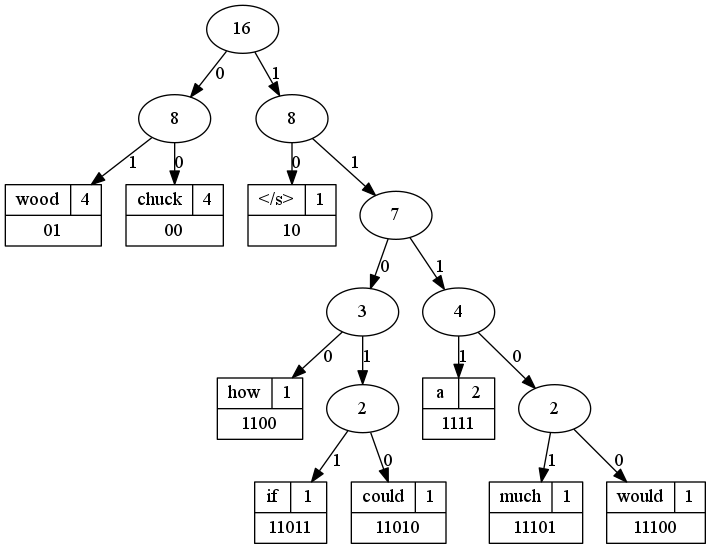
So now we have a nice Huffman tree that provides binary codes for each full word in the vocabulary. Note that we’re encoding full words here. In typical applications of the Huffman coding scheme, we’d be encoding characters. In this case, we want to keep the full words in tact.
part 2: use of the tree
Note that this part of the post still uses the “wood chuck” vocabulary I defined in part 1.
hierarchical softmax?
The goal of this method in word2vec is to reduce the amount of updates required for each learning step in the word vector learning algorithm.
In an un-optimized approach, at every backpropagation step, a matrix with a size of the entire vocabulary (`W`) times the word vector size (`N`) will be updated. This is because of the way in which we are trying to represent the probability of seeing an output word `W_O` given an input word `W_I`.
un-optimized softmax
is the output vector of the training word we want to predict, given , which is the vector of the input word we are using for the basis of prediction (both vectors are initially random, and are learned during training).
This gets a little more complicated when we are using multiple words for the “Skip gram” and “Continuous Bag of Words” methods, but the basic idea is the same.
You can see in the denominator that we have an operation involving all `W` word vectors, hence the inefficiency.
optimization
The “hierarchical softmax” approach is one method proposed to address this inefficiency [2]. Rather than update all words in the vocabulary during training, only `log(W)` words are updated (where `W` is the size of the vocabulary).
How do we cut down the updates? We use the Huffman tree to redefine our probability optimization function:
Couldn’t be simpler!
Okay… this obviously needs some explanation.
more meaning for nodes in the tree
`n(w,j)` describes the j-th node on the path from the root to w
`L(w)` is the length of this path.
This means we’ll have slightly different `L(w)` values for each word:
Using our “wood chuck” example, let’s look at `n(1,j)`. Remember that word 1 is “wood” (see above).
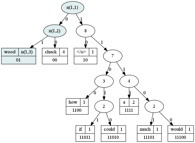
Here we see that `L(1)` is only 3. Our two inner nodes `n(1,1)` and `n(1,2)` describe the walk from root to “wood.” The leaf node at the end of this walk is `n(1,3)`.
Let’s look at the walk to word 4, “how.”
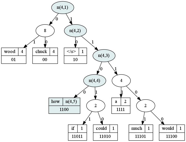
Here we see that `L(4)` is 5. Our inner nodes `n(4,1)`, `n(4,2)`, `n(4,3)` and `n(4,4)` describe the walk from root to “how,” which itself is a leaf at `n(4,5)`.
understanding the probability formula
Let’s talk about the rest of what’s going on in that beast:
`ch(n)` is an arbitrary fixed child of `n` (let’s call it the “left” child)
`[[x]]` is a special function:
These definitions refer to what’s in bold below:
Basically what this says is: “If the next node in the walk to the target word is the left node, use a multiplier of 1. Otherwise, if the next node in the walk to the target word is not the left node, use a multiplier of -1”
All this really does is help nudge the probabilities predicted with the part of the equation in a “left” or “right” direction.
This leads us to the last part of the equation, the vector’s used…
vector representations in hierarchical softmax
In any single-layer neural network, we have two weight matrices. In word2vec, the first matrix is called the “input” or “projection” layer. These are vector representations of input words. They are the inputs (`w`) to the probability formula.
The second matrix is the “output layer.” In the “noise contrastive” model, and in the un-optimized model, the output layer contains another vector representation for each word in the vocabulary.
In the hierarchical softmax approach, the output layer vectors (each column in the output layer) do not represent words, they represent an interaction of the input words with the inner nodes of the Huffman tree.
is the vector representation of the inner unit `n(w,j)`. This is a column in our “output layer” matrix.
`h` is the output value of the hidden layer, which in word2vec, is essentially just a transposed row from our “input layer” matrix.
(Again, a little different with Skip Gram and CBOW, but don’t worry about this for now)
Going back to our probability function, this part is the key:
Each vector in the output layer interacts with the vectors in the input layer (via transformation to the hidden layer) to produce an operand in the probability product.
So each vector in the output layer essentially decides the probability of going left or right in the walk down the Huffman tree at each inner node, given a vector representation of a word provided by the input layer.
Both the input layer vectors and the “probability vectors” in the output layer are adjusted during the learning process.
The adjustments maximize the probability that at some node `n(w,j)` we are going to take a step down the tree toward our expected output word.
For more in-depth description of how word2vec works, please check out Xin Rong’s paper, word2vec Parameter Learning Explained.
references
- [1]Tomas Mikolov, Kai Chen, Greg Corrado, and Jeffrey Dean. 2013a. Efficient Estimation of Word Representations in Vector Space. arXiv preprint arXiv:1301.3781.
- [2]Tomas Mikolov, Ilya Sutskever, Kai Chen, Greg Corrado, and Jeffrey Dean. 2013b. Distributed Representations of Words and Phrases and their Compositionality. In Advances on Neural Information Processing Systems.